MAPHIS — Measuring Arthropod Phenotypes using Hierarchical Image Segmentations

---

Introduction

MAPHIS is a GPL open-source application that allows you to automatically or manually perform hierarchical segmentation of arthropod photos, and to extract various measurements describing the size, shape, colour, or texture properties of their individual body parts.

The application is not limited only to arthropod photos. With a different segmentation plugin or using manual editing, even photos from completely unrelated domains can be processed.

---

Download and installation of MAPHIS

Installing and running on Windows

For Windows users we provide a convenient distribution package at: https://cbia.fi.muni.cz/files/software/maphis/maphis.zip. Extract the contents of the downloaded zip-file at a destination of your choosing and run MAPHIS by executing the file maphis.exe inside the extracted folder.

NOTE: This way of obtaining and running MAPHIS is the most convenient. However, on some machines, you may encounter that the program freezes when clicking on labels in the Labels tree view. This is linked to the way the distribution is generated. As far as we know, this problem is not MAPHIS-specific and is currently out of our hands. If you do encounter this problem, we recommend looking at the alternative ways of installing MAPHIS detailed in the sections below.

Alternative ways of installing MAPHIS

The following sections detail how to install MAPHIS either through the Python Package Index or git. The required prerequisite for both of these ways is to have the Python interpreter installed. You can obtain Python from https://www.python.org/. MAPHIS is compatible with Python versions 3.8 or later, however it was developed and extensively tested mainly with Python 3.8.

Virtual environment

As MAPHIS contains a few dependencies, their versions might clash with versions of the same dependencies that you already may have installed in your Python environment. To prevent this, we recommend installing MAPHIS (and it is generally a good practice for other big projects) in its own virtual environment (see https://realpython.com/python-virtual-environments-a-primer/#why-do-you-need-virtual-environments for further explanation).

The steps below describe how to create a virtual environment using the miniconda manager. Virtual environment management can be also achieved with the modules venv (https://docs.python.org/3/library/venv.html) or virtualenv (https://virtualenv.pypa.io/en/latest/).

1. Download and install miniconda for your operating system from https://docs.conda.io/projects/conda/en/latest/user-guide/install/index.html.

2. Open up Anaconda Powershell Prompt or Anaconda Prompt (Windows) or your terminal emulator (Linux/Mac).

3. In the prompt, create a new virtual environment called maphis with Python 3.8 (you can change the version in python=3.8 as you like, it should be 3.8 or higher, though): conda create -n maphis python=3.8

Alternative 1: Installing from PyPI and running from command line (Linux, Windows or Mac)

In this section we describe how to obtain MAPHIS from the Python Package Index(https://pypi.org/).

Installation

1. Activate the virtual environment: conda activate maphis
2. Install the app: python -m pip install maphis

Running

1. Activate the virtual environment: conda activate maphis
2. Start MAPHIS like so: python -m maphis

Alternative 2: For developers - cloning the git repository

Installation

1. Clone the repository from https://gitlab.fi.muni.cz/cbia/maphis
2. Go to the root directory of the cloned repository
3. Activate the virtual environment: conda activate maphis
4. Install the requirements: python -m pip install -r requirements.txt
5. Install the app in editable mode: python -m pip install -e .

Running

1. Activate the virtual environment: conda activate maphis
2. Go to the root directory of the cloned repository
3. Run: python maphis/__main__.py

Or you can alternatively run MAPHIS with python -m maphis after Step 1.

---

FAQ

A list of questions & answers is maintained here: https://maphis.fi.muni.cz/FAQ/

---

Common Workflow Tutorial

In this manual/tutorial, we will go through a common workflow analysing photos of two bug species, Graphosoma lineatum and Pyrrhocoris apterus (download links are provided below).

We will segment the photos, learn how to manually edit the segmentations, and extract various measurements of individual body parts.

At the end of the tutorial, two advanced topics will be discussed: comparing the body profiles of different specimen groups (which can be used, e.g., when studying mimics and their models, or shape variations in different populations), and quantification of the texture/pattern.

• If you want to work with the photos used in this tutorial, you can download MAPHISTutorialPhotos.zip — this 78 MB archive contains high-resolution photos of the same two species (though not necessarily the same specimens).

• Alternatively, you can download MAPHISTutorialPhotosDownsampled.zip — this 6.6 MB archive contains low-resolution photos for which some functions (such as automatic scale detection) may not perform ideally.

The sets contain photos of Graphosoma lineatum and Pyrrhocoris apterus. The Graphosoma specimens have been included specifically because the automatic segmentation plugin has not been trained to segment photos of this species — you will be able to examine what incorrect segmentations look like, and practice manual editing using the provided tools. In contrast, the automatic segmentation of the Pyrrhocoris photos should be reliable.

---

1. Create a new project

   To work with specimen photos in MAPHIS, you need to have the photos organized in projects. We will start the tutorial by creating one:
   1. Start the MAPHIS application.
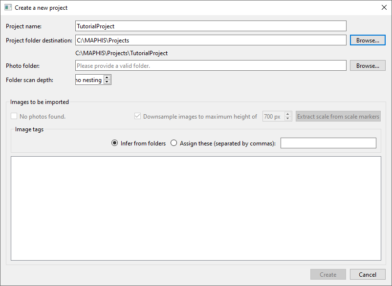
   2. From the menu bar, select File/New project... (Ctrl+N). A “Create a new project” dialog will appear. Fill in the name of the project you want to create (such as “TutorialProject”), and choose where to save the project's data using the upper Browse... button, or type a location (such as “C:/MAPHIS/Projects”) directly:
      
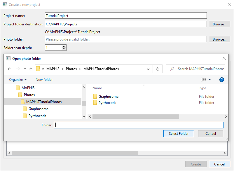
   3. Choose some photos to import into the project: click the lower Browse... button, navigate to a folder containing your photos, and confirm the selection. If the photos in the selected folder are further organized in subfolders, increase the Folder scan depth. In our case, we will navigate to the “MAPHISTutorialPhotos” folder, select it, and set the scan depth to 1, so that photos inside both the “Graphosoma” and the “Pyrrhocoris” subfolders will be used:
      
      (If there were further subfolders inside these, such as “Graphosoma/Male”, “Graphosoma/Female” etc., we would set the scan depth to 2.)
   4. After the photo folder has been selected, a list of photo thumbnails found inside will be displayed:
      
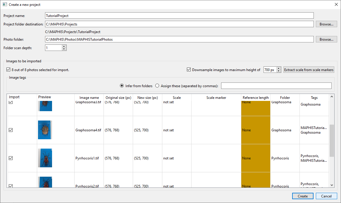
      • Above the photo list, you can choose to downsample all photos to a specified maximum height for the purposes of the application (copies will be created; your original photos will remain untouched). The automatic segmentation plugin supplied with MAPHIS tends to work best on images approximately 700 pixels high.
      • To downsample an individual photo, double-click its New size (px) cell in the list.
      • If your images contain scale markers such as these , scale can be automatically determined by clicking Extract scale from scale markers (this may take a moment, and may fail if the scale bars are too small or too blurred in the photos). If the detection is successful, the detected scale bars will be displayed in the list together with the reference lengths extracted from them (for quick verification). If any of the scale values are incorrect or missing, they can be edited later.
      • To specify the scale of an individual photo, double-click its Scale cell in the list. The process of individual scale setting is described below.
      • Above the photo list, you can also choose how to assign initial tags to your photos. Each photo in a project can have several tags that allow you to organize them into various groups — typical tags would be for instance “Graphosoma”, “Female”, or “FoundAtLocation1”. You can either have the tags assigned automatically based on which subfolder a particular photo was stored in (default), or you can assign a specific set of initial tags, separated by commas, to all photos (such as “Graphosoma, Female”). Tags can also be freely edited later.
      • To set the tags of an individual photo, double-click its Tags cell in the list and enter the tags separated by commas.
      • In the checkbox column on the left, you can select which photos to import, and which ones to skip.
   5. When you have selected the photos you want to import into the newly created project, click Create. More photos can be added to a project later by selecting File/Import Photos... (Ctrl+I).

   ---

2. Browse, adjust, and organize photos in a project

   1. After you create a new project or open an existing one, you will see the thumbnails of all photos in the project on the left side of the screen.
      • To navigate between photos, simply click the thumbnails, or use the arrow buttons below the main photo display.
      • If you need to select multiple photos (for instance to apply a plugin to a specific subset of the photos), you can select multiple photos by Ctrl+clicking, or Shift+clicking to select an interval.
   2. When you hover the mouse cursor over any of the thumbnails, additional controls will appear:
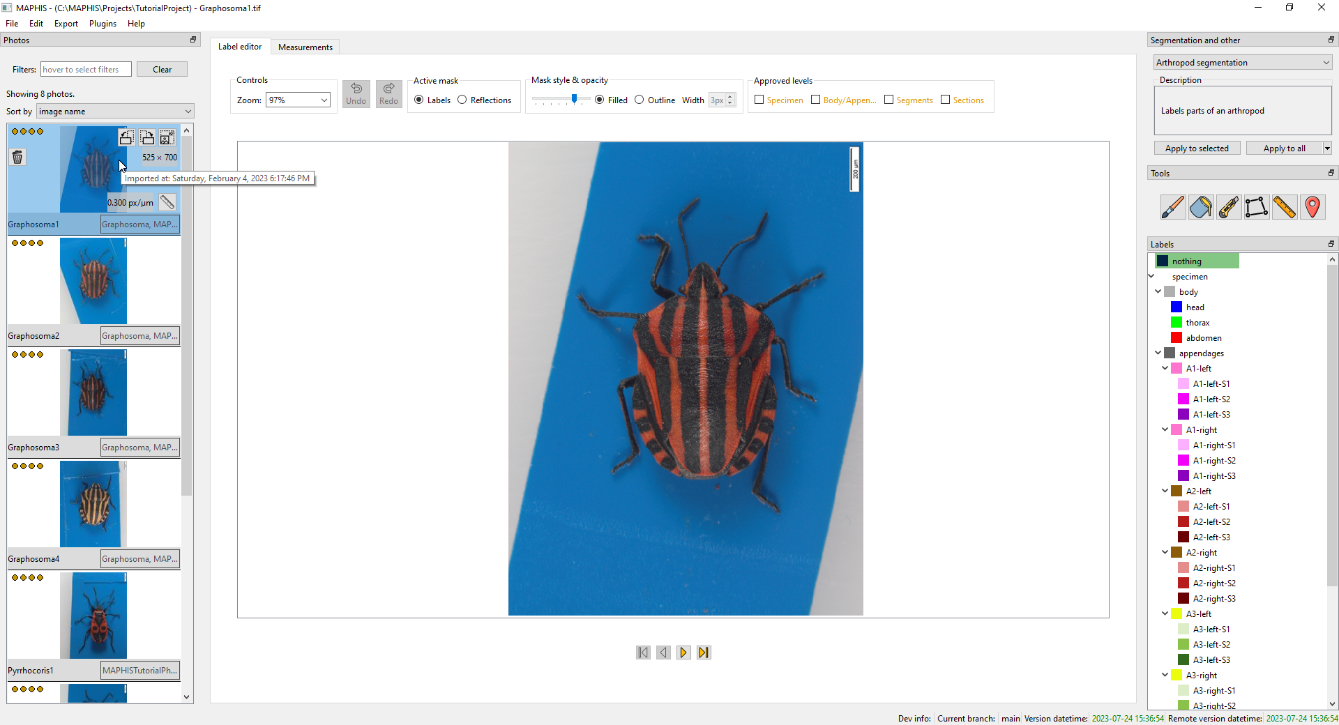      These buttons allow you to:
      • Delete individual photos and associated data (such as segmentations and measurements) from the project.
      • Rotate photos counter-clockwise or clockwise (the supplied segmentation plugin assumes a canonical orientation with the arthropod's head pointing up).
      • Shrink the photo if its pixel dimensions are too large.
      • Set the scale of the photo (if it hasn't been already determined, or if it needs to be corrected).
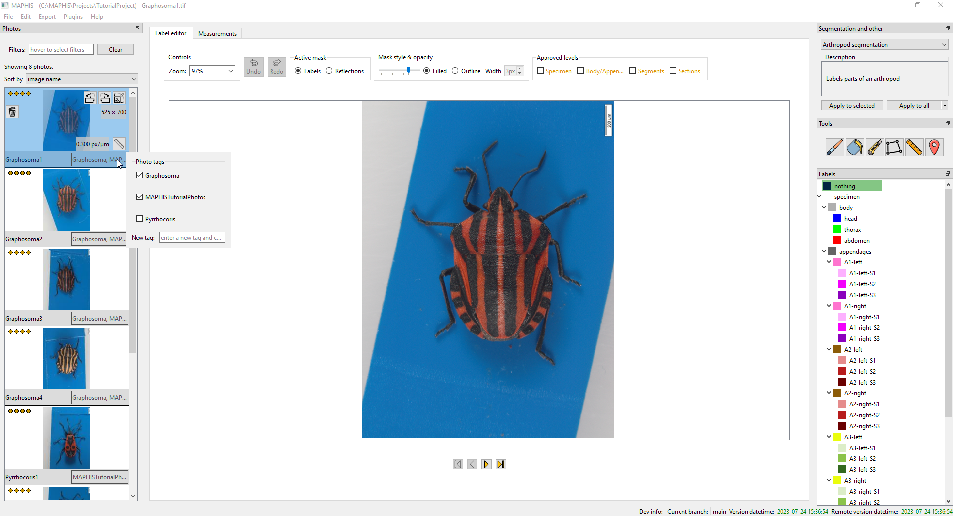
   3. Next to the name of each photo, you can also see a field displaying all tags of that photo.
      • If you hover the mouse cursor over the field, a small panel will pop up and let you add or remove the tags. To add a brand new tag, type it into the text field and press Enter:
        
      • Above the thumbnail list, there is a Tag filter field that allows you to display only the photos with a particular combination of tags. You can use this to view, for instance, only the photos that have the “Pyrrhocoris” tag (or a combination, such as “Pyrrhocoris, Male”):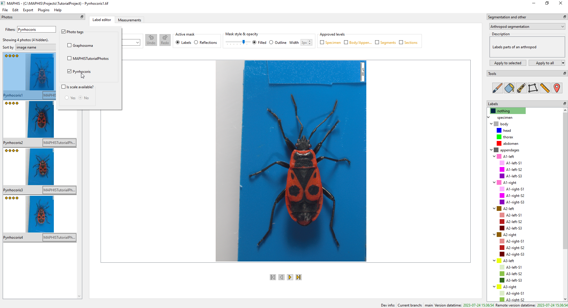
      • You can also filter the photos based on the availability of the scale information.
      • To remove the current filter and show all photos again, click the Clear button next to the filter.
   4. To set a scale of a photo, use the small button with the icon of a ruler in the bottom right corner of a photo's thumbnail. A new window will open.
      • In this window, zoom (scrolling the mouse wheel) and pan (holding the middle button or mouse wheel and dragging) to a scale bar or a ruler present in the photo:
        
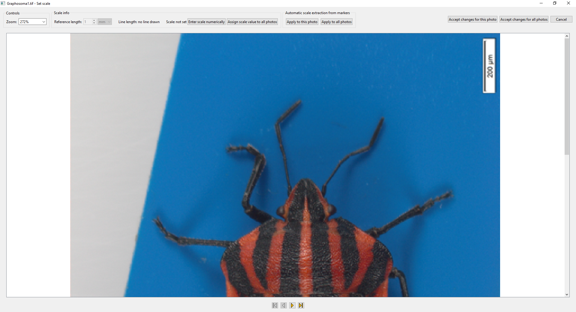
      • After that, draw a line from one end of the scale bar to the other (holding the left mouse button and dragging). Then specify the real-world length of the line you have drawn using the controls at the top (in this case, “200 μm”):
        
      • When you are satisfied with the reference line drawn and the length entered, click Accept changes for this photo to set this scale for this photo, or Accept changes for all photos to set it for all photos in the project.
      • Automatic detection of the scale can be attempted by clicking the buttons in the Automatic scale extraction from markers box (this could have been done also when importing the photos).
      • If you want, you can also specify the scale explicitly with the Enter scale numerically button (this numerically specified scale can also be assigned either just to the current photo, or to all photos in the project).

   ---

3. Use automatic segmentation & detection of reflections

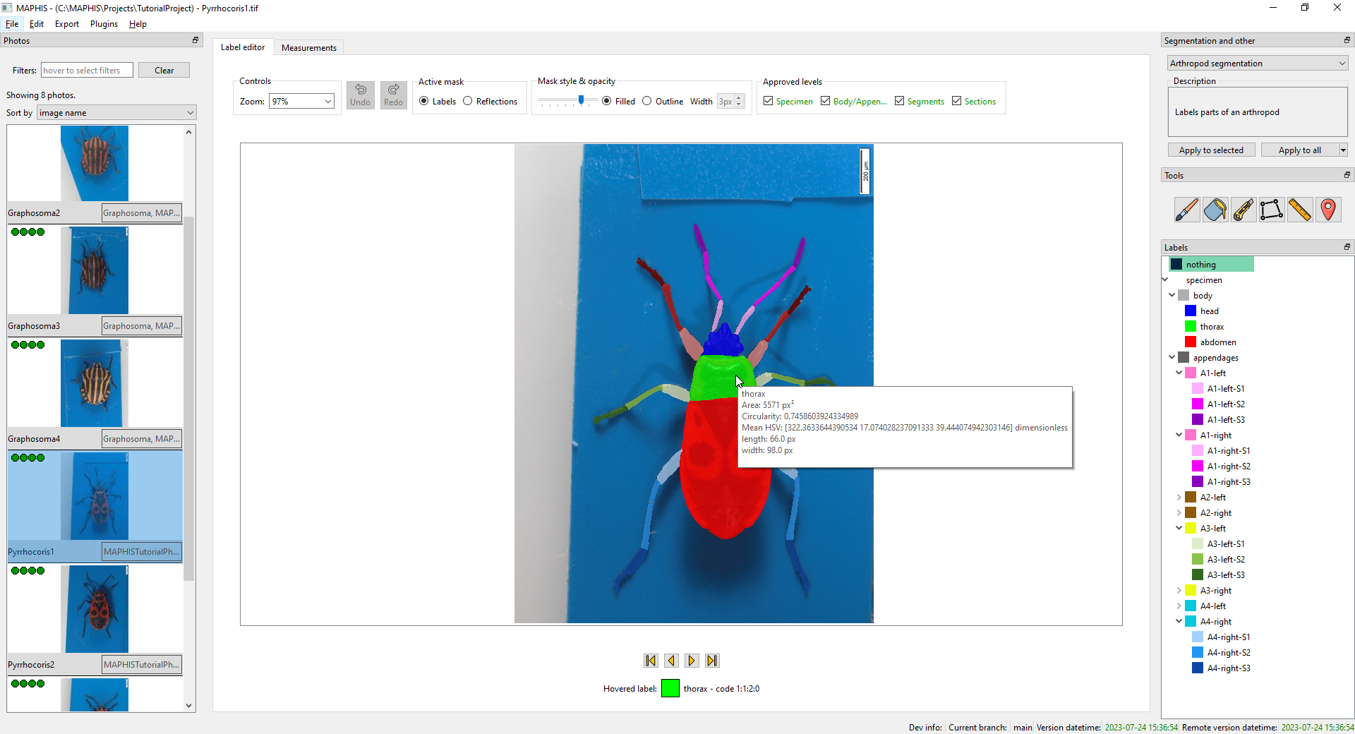
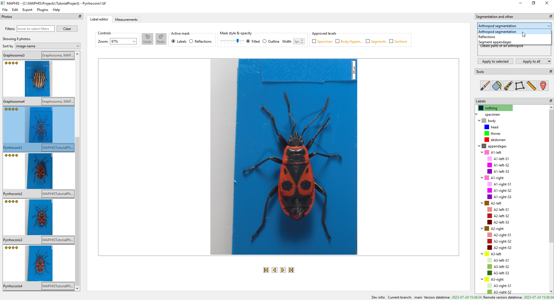
   1. Once all photos are ready (reasonable size and the specimens in a “head upwards” orientation, ideally also with the scale values specified), you can use the automatic segmentation plugin to divide the photo into regions corresponding to individual body parts. MAPHIS is distributed with a segmentation plugin based on a U-Net. To select it, pick Arthropod segmentation from the drop-down list in the upper right corner of the screen:
      
   2. To start the computations, click the Apply to all button below the drop-down list. Alternatively, you can apply the segmentation only to the currently selected subset of the photos (often just the one photo being displayed); or, using the small drop-down arrow, to all those photos that do not have a segmentation yet. Once started, the segmentation may take some time to finish.
      
      After the segmentation is computed, you can examine the regions into which the photo has been divided:
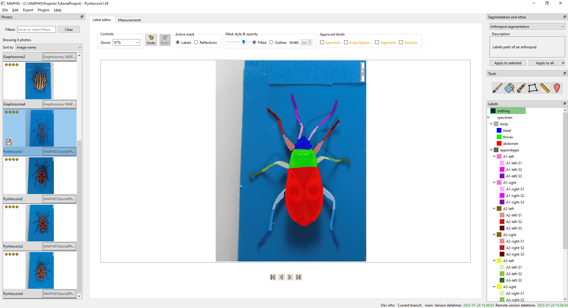      You can adjust the display by using the Mask style & opacity controls above the photo.
   3. Often, the photos may contain areas where glare or light reflections are visible. Those areas can still be parts of the specimen mask, but the colour information there is unreliable (i.e., not suitable for colour or texture analysis). To detect such areas in a segmented photo, you can use the supplied Reflections plugin from the same drop-down list, again using Apply to all:
      
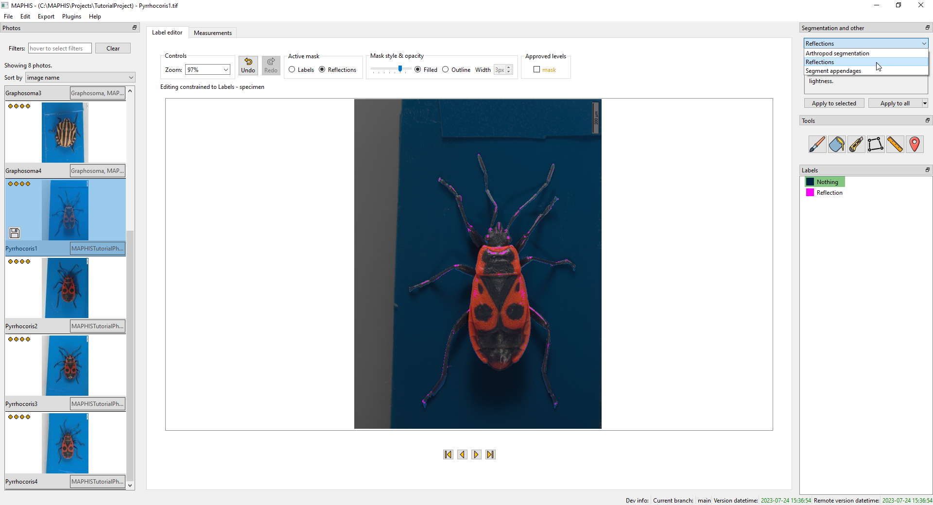
      • Note that the detection of reflections works only within the mask of a specimen. That means that the photo has to be segmented first. Otherwise, no reflections will be marked.

      In the Active mask panel above the photo, you can switch between the display of the individual specimen regions (Labels), and the reflections (Reflections; here, the areas with reflections are indicated with purple, unless otherwise specified).

   4. An important aspect of the segmentation is its hierarchy, which specifies the relationship between individual body parts.
      • By default, the photo is divided into the background, and the specimen. The specimen is divided into the body, and the appendages. The body is divided into head, thorax, and abdomen. And each appendage is divided into three segments. The whole default hierarchy is shown here:
        
      • Each region is indicated by a different “label”. The labels may or may not be shown in different colours; in the default hierarchy for instance, appendages on the left and on the right side have the same colours, but the left and the right version of each are two distinct regions.
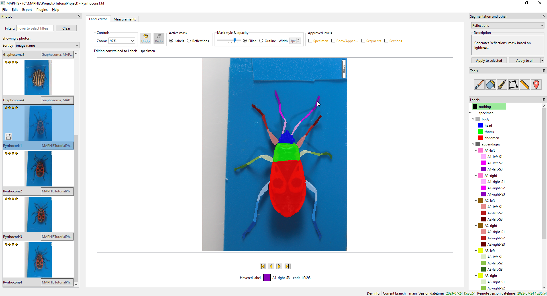
      • You can quickly examine what label each part of the photo has by hovering the mouse cursor over the photo and looking at the status text below. Here, for instance, the mouse cursor is hovering over the tip of the right antenna, which has the “A1-right-S3” label, and is shown in dark purple:
        
   5. You can examine different levels of the hierarchy by clicking the individual labels in the list on the right. When you click a label, the main view will switch to the lowest hierarchy level that contains that label.
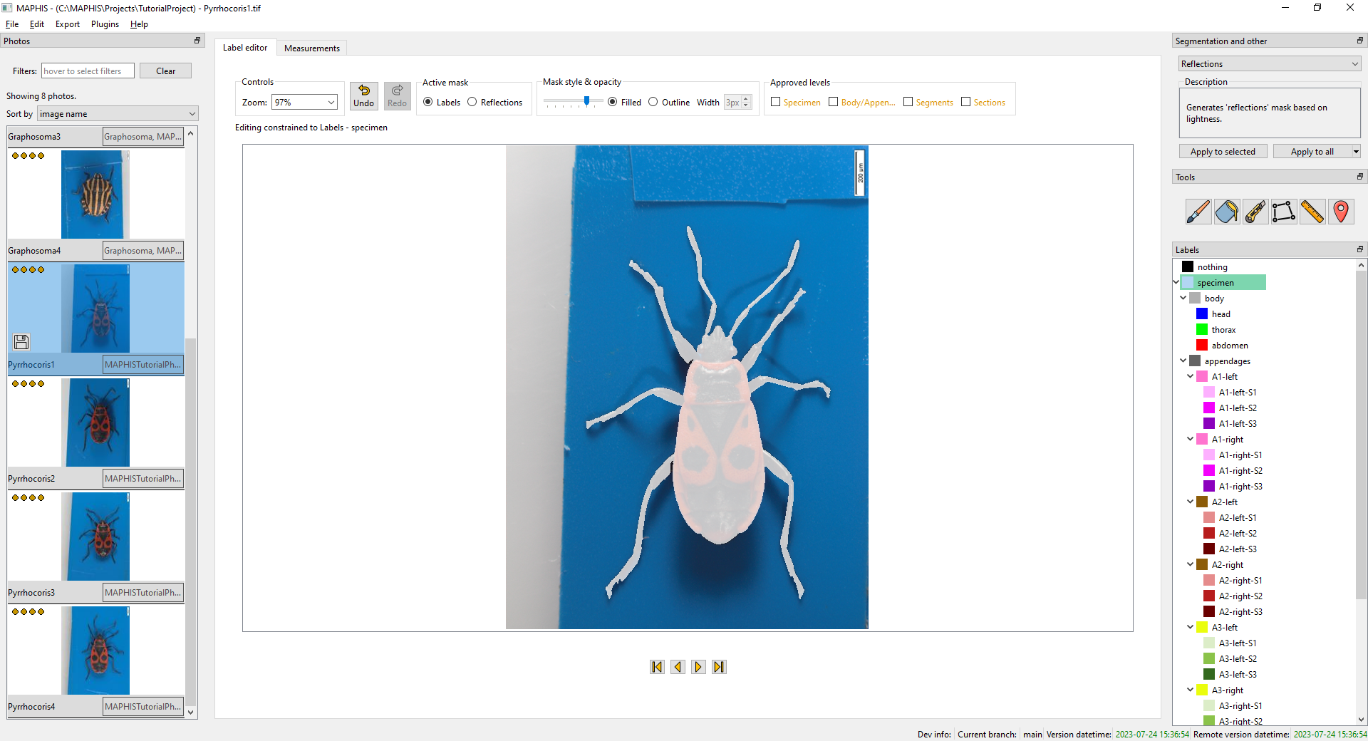
      • When you click the specimen label, you will see the photo segmented into the specimen and the background:
        
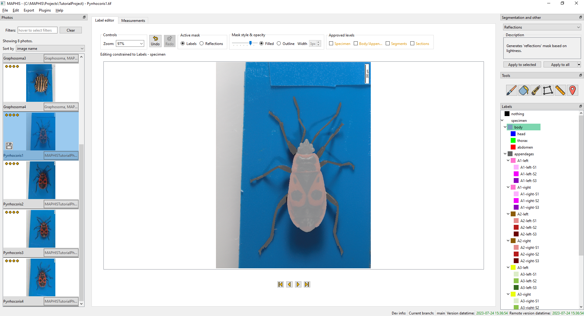
      • When you click the body or appendages labels, you will see the specimen divided into the body and the appendages:
        
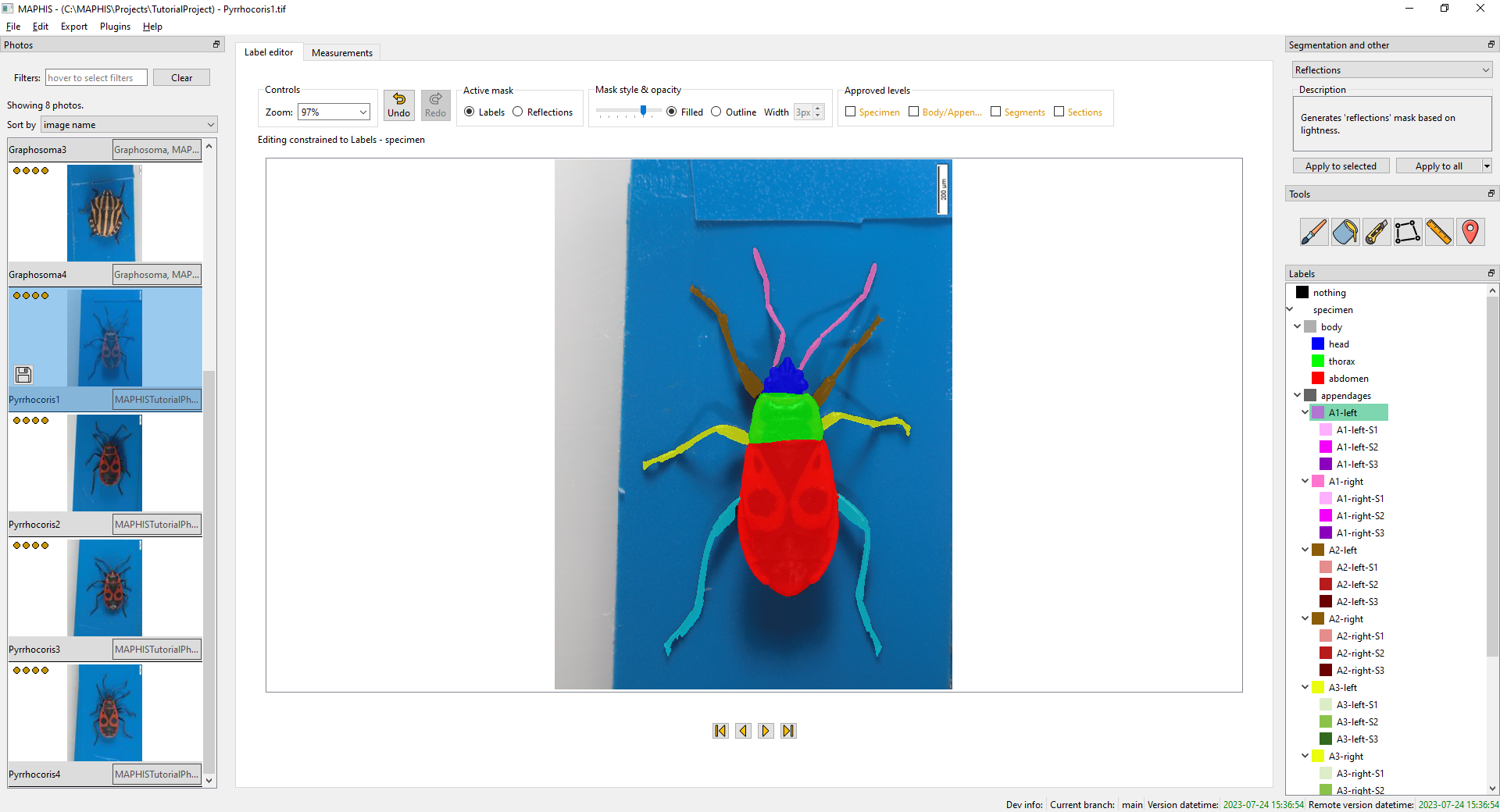
      • When you click a label of an individual whole appendage, such as A1-left, you will see the photo segmented so that each appendage forms one region:
        
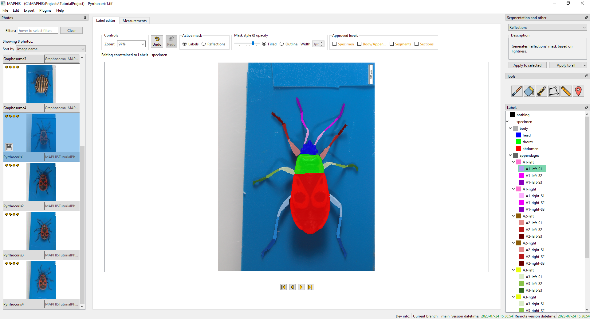
      • When you click a label of an appendage segment, such as A1-left-S1, or the head, thorax, or abdomen labels, you will see the photo segmented at the finest hierarchy level:
        
   6. If you want, you can change the displayed colours and names of the labels by double-clicking them in the list on the right, and using the dialog that pops up:
      
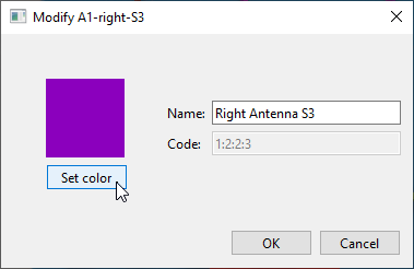
      When the Active mask is set to Reflections, you can use this to change the colour used to indicate the reflections.

   ---

4. Make manual adjustments

   After running the automatic segmentation, it is possible to manually edit the segmentation masks in case any corrections are necessary. It is also possible to create an entire segmentation from scratch this way — that can be useful when working with photos for which no automated segmentation plugin is available (e.g., photos of plants, fish, or even photos from entirely different domains, such as material science).

   You can manually edit both the hierarchical segmentation of a specimen into regions, and the reflection mask.

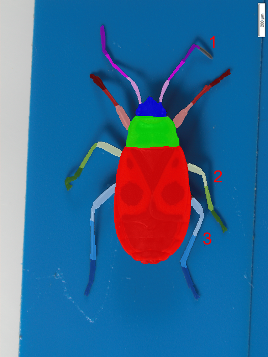
   We will demonstrate the edits on the segmentation of the Pyrrhocoris2.tif photo. We see that the tip of the right antenna hasn't been detected properly (area labeled as “1”), and the subdivision of some legs into the segments needs improvement (areas “2”, “3”):
   
   (You can zoom by scrolling the mouse wheel, and pan around by holding the middle button or mouse wheel and dragging.)

   ---

   Editing tools & constraint system

   To make manual edits, the application offers a set of tools that should be familiar from common image editing programs. The tools can be selected from this toolbar on the right side of the window:
   
   

   The application offers a simple “constraint system” that allows you to limit any edits to within a specified area, helping you “stay inside the lines” as in a coloring book. We will demonstrate its functionality in a moment, together with the Polygon tool.

   When editing, you should generally select the “active” or “current” label by clicking on it in the region hierarchy panel. To fix the missing tip of the right antenna, we will need to select the A1-right-S3 label:
   
   

   (Be careful: the selected label is not the same as “color” — for instance, the A1-left-S3 and A1-right-S3 labels might both be displayed using the same purple color, but they are two distinct labels, and must be treated as such.)

   When a tool is active, you can also “pipette” a label directly from the segmentation mask by right-clicking the mouse. After the right-click, you should see the selection change in the hierarchy panel. Right-clicking the background will select the nothing label.

   ---

   1. The Brush tool is selected using this icon:

      We will correct the tip of the right antenna (area “1”) with the Brush. Click the tool icon, and set Radius below it to something small, like 3. You can also change the Brush radius by holding down Shift and scrolling the mouse wheel.

      If you haven't selected the A1-right-S3 label yet, do it either by clicking it in the hierarchy panel, or by right-clicking the existing part of the antenna's last segment to “pipette” it. The cursor should now indicate the selected label and the brush size:
      
      

      Draw the tip of the antenna as you would in any image editing program. If you make a mistake, you can use Ctrl+Z and Ctrl+Y as “undo” and “redo” (these work also with other tools). To shrink a region, mark a part of the photo as background using the nothing label (you can “pipette” it by right-clicking the background).

      (In general, you should always use the most specific applicable label of the hierarchy, such as A1-right-S3 or head. It is however possible to use also the less-specific ones, if needed. You can, for instance, use the body label to mark the pixels that should belong to the specimen's body, but shouldn't be for some reason counted as part of its head, thorax, or abdomen.)

   2. The Bucket tool is selected using this icon:

      When using the paint bucket, you can fill a contiguous area of the segmentation mask with the active label.

   3. The Knife tool is selected using this icon:

      This tools lets you slice the regions using straight cuts of a specified width. We will correct the subdivision of the middle right leg (area “2”) into segments by using the Knife and the Bucket to expand the middle segment of the leg.

      First, select the Knife tool. Then pipette the A3-right-S2 label by right-clicking the middle segment of the leg. Then draw a cut across the joint by dragging the mouse:
      
      

      Finally, select the Bucket tool and click the area between the cut and the rest of the middle leg segment to change its label from A3-right-S1 to A3-right-S2:
      
      

   4. The Polygon tool is selected using this icon:

      The Polygon tool lets you fill a polygonal area by marking its circumference with a combination of clicking (to place individual vertices) and dragging/drawing (to draw free-hand parts).

      We will demonstrate this tool by fixing the subdivision of the bottom right leg (area “3”). To do that, we will also use the application's “constraint system”. We will need to expand the leg's middle segment:
      
      

      First, select the Polygon tool and the A4-right-S2 label corresponding to the middle segment of the leg. We see that the leg itself is segmented correctly, only its subdivision needs to be adjusted. To limit any further edits to within the bottom right leg, move your mouse to the A4-right label in the region hierarchy panel, and click the Set constraint button that appears next to it:
      
      

      The display will indicate that any edits made now will be limited to within the A4-right region, i.e., the bottom right leg:
      
      

      With the A4-right-S2 label selected, and the constraint set to A4-right, draw any polygon that fixes the leg subdivision. You don't need to care about intersecting any other regions. You can combine clicking and dragging. To finish drawing the polygon, double-click:
      
      

      To remove the constraint, click the Remove constraint button in the hierarchy panel.

      Notes on efficient using of the constraint system:

      The constraint system can be used together with any tool. For instance, the same result as above could be achieved also with a single click using an oversized Brush:
      
      

      If you want to quickly switch between different constraints, you can point the mouse cursor at any part of the photo, hold Ctrl, and scroll the mouse wheel. This will cycle between all constraint levels applicable to this part of the photo. For instance, when pointing at A4-right-S2, the constraint will cycle between none, specimen, appendages, A4-right, and A4-right-S2:
      
      

   5. The Ruler tool is selected using this icon:

      This tool is not used for editing, but for quick measurements. To measure a distance, select the Ruler and drag a line from one point to another. If you tick the Multi-ruler box, you can place multiple rulers in the photo and see their total length as Total measurements. Right-clicking removes all rulers.
      
      

   6. The Landmarks tool is selected using this icon:

      This tool is not used for editing, but for specifying arbitrary points of interest in the photos, which are saved together with your project. To place a landmark, select the tool and click anywhere in the photo. You can also move existing landmarks by dragging them. Each landmark has its [X, Y] coordinates within the photo, and its label, which you can select from a pre-made set, or type in your own, such as “Tip of the left antenna”.
      

      When you later export computed measurements, the landmark coordinates will be exported too, and you will be able to do processing such as calculating their pairwise distances, etc.
      
      

   ---

   Indicating approvals

   To keep track of which photos have had their segmentations examined and manually corrected, you can mark each photo with the “approval” buttons above the main view:
   
   

   Each button corresponds to one level of the hierarchy. To indicate that you consider the segmentation up to a certain hierarchy level “satisfactory” or “done”, simply tick the corresponding box. The approval status of each photo is indicated with small icons in the corner of its thumbnail.

   In the following example, the Specimen level of the Pyrrhocoris1.tif has been approved, but its division into Body/Appendages (and further) is still marked as “work in progress”. Pyrrhocoris2.tif has been approved except the finest subdivision of the appendages into sections, and Pyrrhocoris3.tif probably hasn't been checked yet:
   
   

   Be careful: editing the segmentation can invalidate the approvals. After any edits, it is good to verify if the approvals still reflect your satisfaction with the segmentation.

   ---

   Editing the whole segmentation hierarchy

   You have seen that you can adjust the name and the colour of each label in the hierarchy (allowing changes such as renaming “A1-left” to “Left Antenna”). The hierarchy itself is defined by the plugin that created the segmentation.

   However, if you wish to manually draw a segmentation of a specimen type for which no segmentation plugin exists, you can define your own region hierarchy. To do this, right-click a node in the hierarchy tree, and click Remove label or Remove label and children to remove that region from the hierarchy, or click New child label to add a new sub-region with a desired name and colour. (Note that the root of the hierarchy cannot be removed, and the hierarchy cannot be deeper than 4 levels.)

   For instance, if you wanted to manually segment microscopic cell images and then use the program to perform some measurements, you could define a hierarchy with a region called “cell”, which would divided into “cytoplasm” and “nucleus”, etc.

   ---

5. Take and export measurements

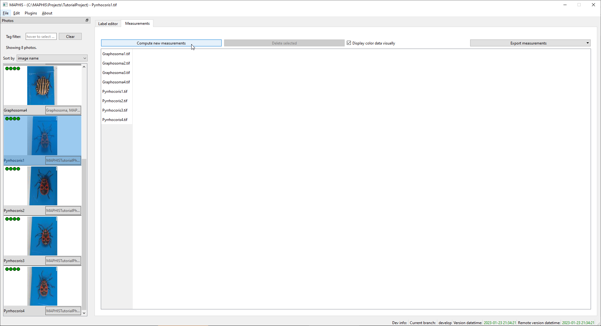
   1. When the photos are segmented to your satisfaction (which you can indicate using the Approvals described above), you can proceed to taking the measurements. To do this, switch to the Measurements tab. Initially, it contains an empty table:
      
      

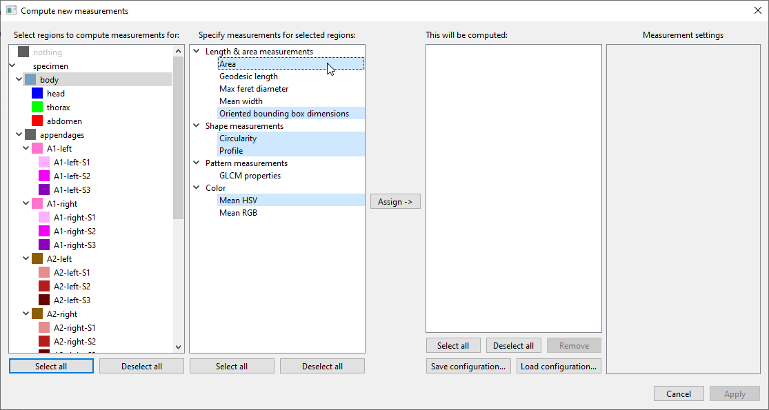
   2. After clicking Compute new measurements, a new window will open. Here you can select which measurements should be computed for which regions. For instance, you can select body in the list of regions, and Area, Oriented bounding box dimensions, Circularity, Profile, and Mean HSV in the list of available measurements:
      
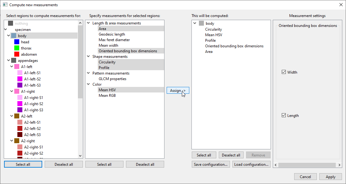
      Then click Assign -> to add these combinations to the list of measurements to be computed:
      
      

   3. This can be repeated until you have specified all “region + measurement” combinations you want computed. Different measurements make sense for different regions. For instance, Geodesic length is useful to measure the length of appendages, because it measures the regions along the centerline, taking any bends into account. For a more compact region such as body, Oriented bounding box dimensions would be more appropriate. The full list of available measurements with explanations is provided below.

      In this tutorial, we will also select Geodesic length and Mean width for each of the individual appendages A1-left through A4-right, and GLCM properties (measuring pattern/texture) for abdomen. If any of the selected measurements have any parameters, you can adjust them in the rightmost panel. In our example, tick contrast in the GLCM properties panel to include this property in the results:
      
      

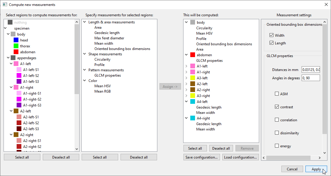
      If you want to re-use a list of “region + measurement” combinations that you have prepared, you can use Save configuration... and Load configuration.... To remove a combination from the list, select it and click Remove.

   4. When everything is set up, click Apply to perform the selected measurements. Provided the segmentation was correct, you should see something like this after the computation finishes:
      
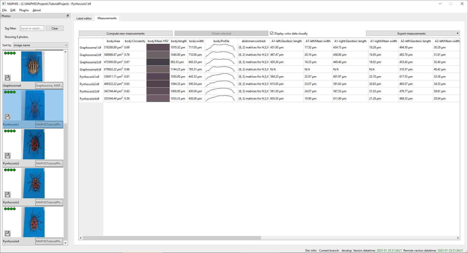
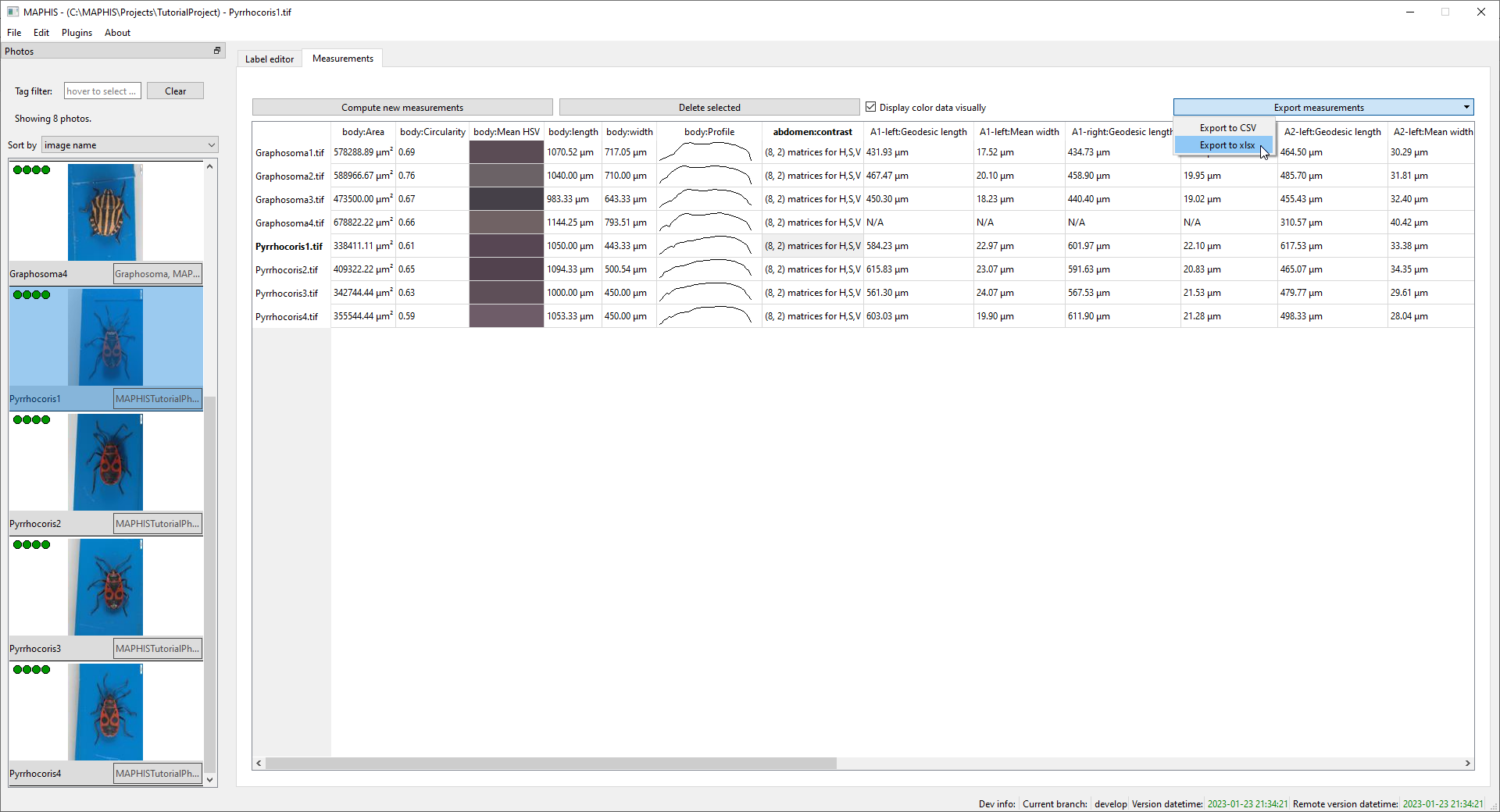
      In this view, we can briefly examine the results. Already just looking at the table, we can see that, for instance:

      • The Pyrrhocoris specimens were smaller than the Graphosoma ones.
      • The bodies of the Graphosoma specimens were slightly more circular than those of the Pyrrhocoris specimens (which were narrower).
      • The mean color of the Graphosoma specimens was more varied.
      • The body profile of the Graphosoma specimens differs from the Pyrrhocoris ones, with a narrowing between the thorax and the abdomen (head is to the left).
      • No antennae were segmented for one of the Graphosoma specimens.

   5. To examine a compound measurement result in detail, double-click its cell. In our example, we can do this with the Profile vectors, or with the matrices that form the results of the Contrast measurement:
      
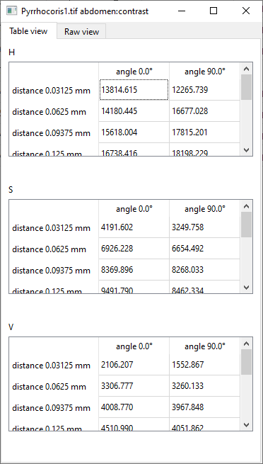
      (In the GLCM properties measurements like Contrast, the results quantify the pattern in different directions and over different distances, forming a matrix for each of the Hue, Saturation, and Value channels. We will show how these values can be processed and understood below.)

   6. Finally, you can export the table of all computed measurements and landmark positions to a spreadsheet format, to process the data in other software. Click Export measurements, and then choose whether you want to save the results in the .xlsx format for Microsoft Excel and compatible, or as .csv (comma separated values) for more general processing (e.g., by your own scripts):
      
      

   ---

6. Available measurements

   Size (in pixels or SI units)

   Area	Total area of the region.
   Geodesic length	Along-the-centerline length. Suitable for elongated regions such as appendages (takes any bends into account).
   Max feret diameter	Maximum “caliper” size of the region.
   Mean width	Mean width. Suitable for elongated regions such as appendages.
   Oriented bounding box dimensions	Size of the minimum-area bounding box of the region. Suitable for more compact regions such as the specimen body, its head, etc. In the parameter settings, select which dimensions to include: width is the dimension closer to horizontal, length is the dimension closer to vertical.

   Shape

   Circularity	Value from 0.0 to 1.0, where 1.0 means a perfect circle.
   Profile	Vector of 40 distances between the region outline and its main axis, spaced at regular intervals, describing the overall shape of the region. When exported to a spreadsheet application, you can plot these values as a graph, with results similar to the small graphic preview shown in the Measurements table. The profiles can also be used for more elaborate comparisons directly inside MAPHIS (see the next chapter).

   Pattern/texture (These measurements ignore pixels in areas marked as reflections.)

   GLCM properties

   Properties calculated from a Gray-Level Co-occurrence Matrix (GLCM), based on “Haralick, R. M., Dinstein, I., & Shanmugam, K. (1973). Textural Features for Image Classification. IEEE Transactions on Systems, Man and Cybernetics, 3(6), 610–621. https://doi.org/10.1109/TSMC.1973.4309314”. To use these, you should select which properties you want to compute, and then specify a list of distances and a list of angles. Distances in mm should contain a list of distances separated by commas, such as “0.03125, 0.0625, 0.09375, 0.125, 0.15625, 0.1875, 0.21875, 0.25”. Angles in degrees should contain a list of angles separated by commas, such as “0, 90” (values should come from the [0, 180) interval; angle 0 is “to the right”). For each selected property, the result will consist of three matrices: one for each of the Hue, Saturation, and Value colour channels. In each matrix, the values express the relationship between pixels that are a certain distance apart in a certain direction. For instance, you can examine the average contrast of pixels that are 0.125 mm apart in horizontal direction (0°). An example that should help you understand this more intuitively, including a useful application, will be provided in a chapter below. The available properties are: ASM: Angular second moment, a measure of homogeneity. Contrast: Amount of local variation. Correlation: Measure of grey-level linear dependencies. Dissimilarity: Weighted sum of absolute grey-level differences. Energy: Square root of ASM. Homogeneity: Inverse difference moment.

   Colour (These measurements ignore pixels in areas marked as reflections. Also note that “averaging” colours works differently in different colour models, so measurements using the HSV and RGB models shouldn't be mixed together.)

   Mean HSV	Mean Hue, Saturation, Value colour values.
   Mean RGB	Mean Red, Green, Blue colour values.

   ---

7. Advanced measurements: Profile fusion and comparison

   Here we will show how the computed profiles (most commonly body profiles) of multiple specimens can be combined and compared. Comparing the body shapes of Graphosoma and Pyrrhocoris specimens this way is a bit artificial task, but the same process can be used to compare, e.g., the body shapes of certain ants and ant-mimicking spiders.

   To do this, we will need the body profile measurements that we computed earlier. For the sake of the example, we will also update the tags of the photos. To simulate that we want to compare specimens originating from two different locations, two of the Graphosoma photos will get a “FromLocationA” tag, and the other two will get “FromLocationB”. We will then do the same with the Pyrrhocoris photos.
   
   

   If we want to compare groups of profiles, we first need to compute a “median profile” for each group, and compare those — such as “median Graphosoma” vs. “median Pyrrhocoris”, or “median Pyrrhocoris from location A” vs. “median Pyrrhocoris from anywhere”.

   The issue with comparing or combining the computed profiles directly (e.g., in a spreadsheet program) is that there are inter-specimen differences that do not correspond to the general body shape of a species, but to individual variations of size. To mitigate this, the profiles in each group first need to be aligned:
   
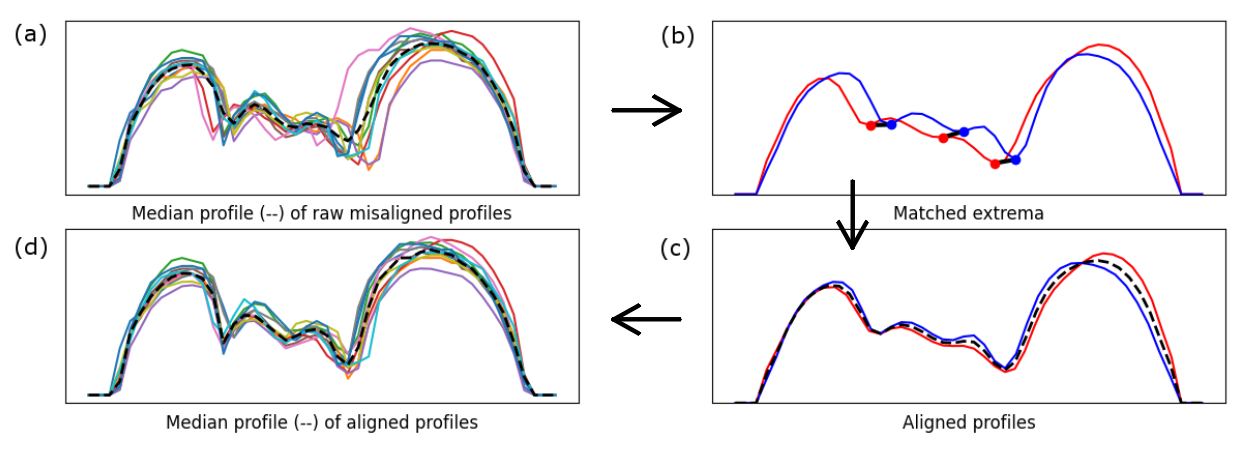
   Figure (a) shows a set of raw, misaligned profiles (in this case, an ant Opisthopsis haddoni). Figures (b) and (c) show how matching extrema (body constrictions) are identified in the profiles, and how the profiles are aligned to match more closely. Figure (d) then shows the set of profiles after they have been aligned. If we compare the median profile (dashed line) of the misaligned set (a) with that of the aligned set (d), we can see that the alignment helps to preserve the body constrictions, which could otherwise be “smoothed out”.

   The process described above can be used within MAPHIS. To start, select Plugins/Profile fusion from the menu. A new window will open:
   
   

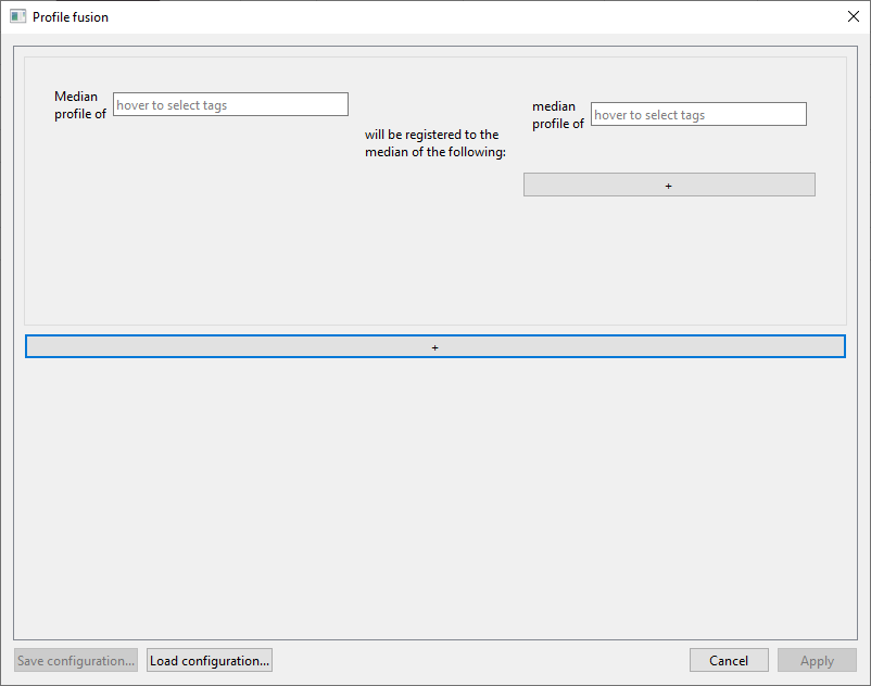
   We will want to compare the Pyrrhocoris specimens from location A with those from location B. To compare them correctly, we should map/register both of these groups to a common space. We will do this in two steps:

   • Compute the median profile of Pyrrhocoris from location A and map/register it to the median profile of all Pyrrhocoris specimens.
   • Compute the median profile of Pyrrhocoris from location B and map/register it to the median profile of all Pyrrhocoris specimens.

   Move the mouse over the left field that says “hover to select tags”, and check Pyrrhocoris and FromLocationA:
   
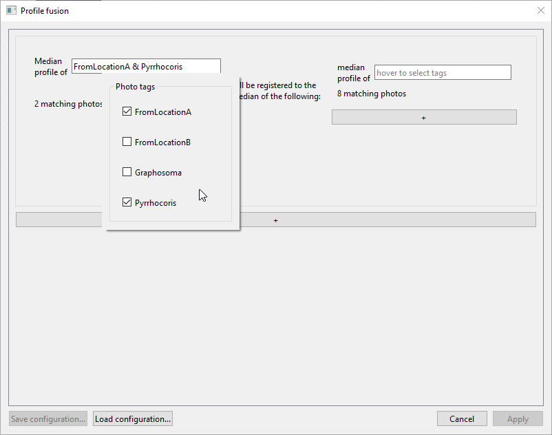
   In the right field, check only Pyrrhocoris. The window should now look like this, with the first registration task being “Median profile of FromLocationA & Pyrrhocoris will be registered to the median of the following: median profile of Pyrrhocoris”:
   
   

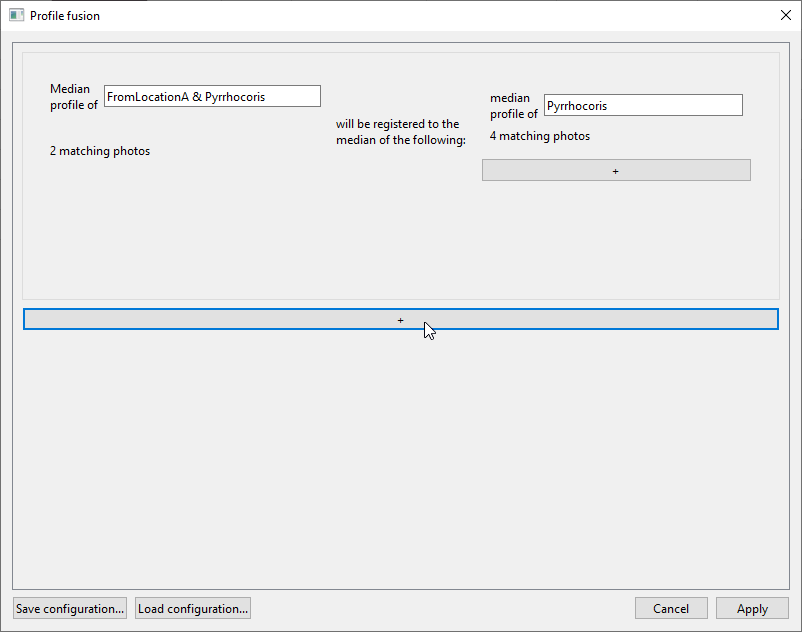
   To add the second task, click the long + button beneath the first task panel. In the second task panel, select Pyrrhocoris and FromLocationB in the left field, and Pyrrhocoris in the right field. The window should now look like this, with the second registration task being “Median profile of FromLocationB & Pyrrhocoris will be registered to the median of the following: median profile of Pyrrhocoris”:
   
   

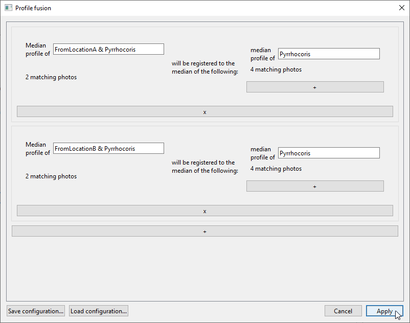
   If you want to re-use the configuration you have set up in this window, you can use Save configuration... and Load configuration....

   When you click Apply, the results will be saved in a registered_profiles/profiles.xlsx file in the project folder.

   The first sheet of the document will contain the raw median profiles from all tasks (“median Pyrrhocoris from location A”, “median Pyrrhocoris from location B”, and two instances of “median Pyrrhocoris”).

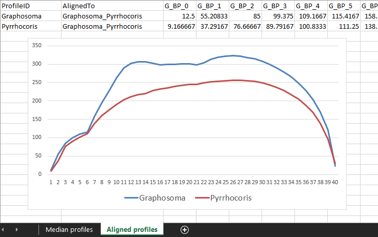
   The second sheet, Aligned profiles, will contain the important results: the profiles mapped to the desired space. In this case, there will be “median Pyrrhocoris from location A mapped to median Pyrrhocoris”, and “median Pyrrhocoris from location B mapped to median Pyrrhocoris”. These aligned profile values can then be plotted or compared with one another easily:
   
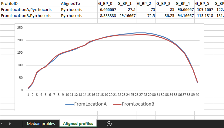
   (Admittedly, these do not have very exciting profiles.)

   ---

   We may also want to compare profiles from completely different groups of photos, which do not share tags. For instance, we can compare the Pyrrhocoris profiles to the Graphosoma ones by mapping both groups to their common median profile — i.e., to the median of (median Pyrrhocoris) and (median Graphosoma). To specify this “median of several different medians” on the right side, use the short + button below the right field in a task panel:
   
   

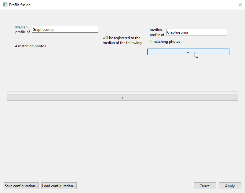
   When everything is set correctly for comparing the Graphosoma and Pyrrhocoris profiles, the window should look like this:
   
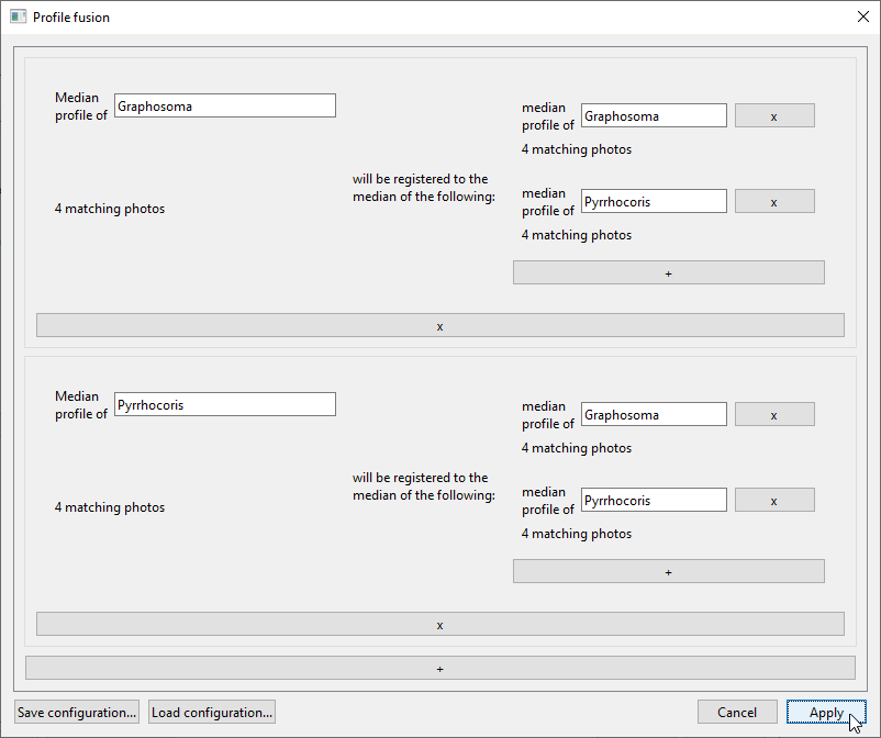
   The tasks specified in this window are:

   • “Median profile of Graphosoma will be registered to the median of the following: median profile of Graphosoma and median profile of Pyrrhocoris”
   • “Median profile of Pyrrhocoris will be registered to the median of the following: median profile of Graphosoma and median profile of Pyrrhocoris”

   After the registration is done, we can again visualize the aligned profiles in the spreadsheet:
   
   

   ---

8. Advanced measurements: Quantifying patterns using GLCM properties

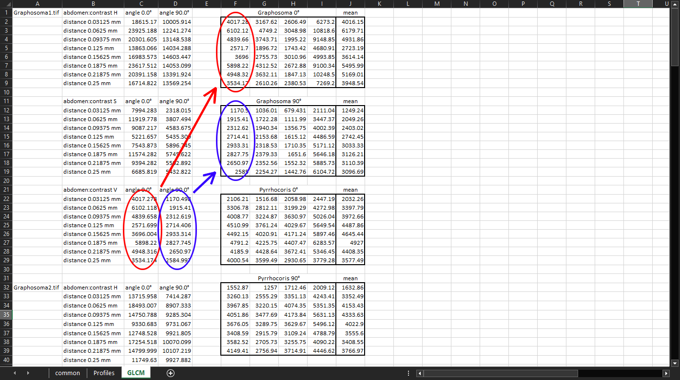
   In this example, we will show how the GLCM properties measurements can be used to quantify the patterns. We will be using the measurements we computed previously: GLCM contrast of the abdomen region, computed with Distances in mm set to “0.03125, 0.0625, 0.09375, 0.125, 0.15625, 0.1875, 0.21875, 0.25”, and Angles in degrees set to “0, 90”. We will export the measurements into a “.xlsx” file and open it in a spreadsheet application. The GLCM properties are on the third sheet:
   
   

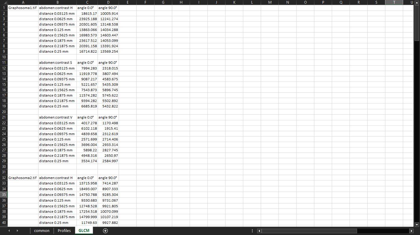
   The C22 cell, for example, says the following (hover the mouse over individual parts of the sentence to see which cell they come from): “In the V channel of Graphosoma1.tif abdomen, pairs of pixels that are 0.03125 mm apart in the horizontal (0°) direction have the average contrast of 4017.278”.

   We will now compare the contrast of the horizontal and the vertical components of the pattern (that is why we picked the angles of 0° and 90°, respectively). For our purposes, the most useful values will be those in the V (Value) colour channel, which correspond to the brightness of the pixels.

   We will now compile four tables:

   • V values for the 0° angle for all Graphosoma specimens.
   • V values for the 90° angle for all Graphosoma specimens.
   • V values for the 0° angle for all Pyrrhocoris specimens.
   • V values for the 90° angle for all Pyrrhocoris specimens.

   For each table, we will also calculate the mean values:
   
   

   Now we can plot the calculated mean values and interpret the results. We can clearly see that in the horizontal direction (angle 0°), the contrast of the Graphosoma specimens depends on how far two pixels are apart. Specifically, the contrast is highest between pixels that are 0.0625 mm apart horizontally, and then again between pixels that are 0.1875 mm apart. The lowest contrast tends to be between pixels that are 0.125 mm apart horizontally:
   
   

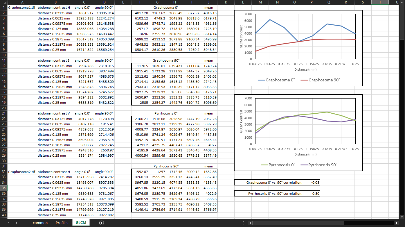
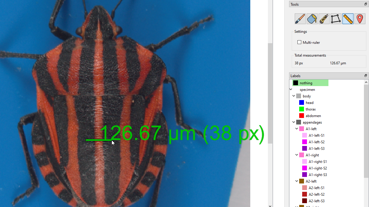
   Since we don't see any similar feature in the vertical (90°) Graphosoma series, this suggests that the abdomen of the Graphosoma specimens is vertically striped. We can even infer that the most common distance from the center of one stripe to the center of the next stripe of the same colour is approximately 0.125 mm. We can check this by using the Ruler tool and measuring it manually in MAPHIS:
   
   

   If we calculate the correlation between the 0° and 90° series for each species, we can even sum up these features into a single number.

   In the Graphosoma specimens, the correlation value of -0.08 shows that the horizontal and vertical components of the pattern are quite different — i.e., that the pattern is directional, such as stripes.

   In the Pyrrhocoris specimens, the correlation between the horizontal and vertical series is 0.8, indicating that any two pixels that are a certain distance apart tend to have the same relative contrast regardless of whether they are spaced horizontally, or vertically — i.e., that the pattern is not as directional.

   ---